Introduction to Algorithms - Chapter 2 (Part 1)

• Introduction
  • Pseudocode
  • Insertion Sort
• Correctness of Insertion Sort
• Interesting Problems/Algorithms
• More to come!

Introduction

Let’s focus on the first problem introduced in the previous chapter, the sorting problem.

Let us examine an algorithm to solve this problem, called insertion sort. We then take the help of this algorithm to lay the framework of analysis of other algorithms.

But before that, we need to know what pseudocode is.

Pseudocode

All algorithms in this book are expressed in something called pseudocode. It is similar in many respects to C++ (Or C/Pascal if you’ve seen them, all of these language share similar syntax), the only difference being that sometimes the authors might swap actual code with English sentences to be more concise.

One exception (that you will probably find in the pseudocode for insertion sort) is that when you write A[j] in this language, it means “The $j^{th}$ element of the array A”, when in C/C++ it means “The ${j-1}^{th}$ element of the array A”.

Since now we have the utmost basic stuff down, let’s get to the first algorithm.

Insertion Sort

Input: A sequence of n numbers $\langle a_1, a_2, a_3, \ldots, a_n \rangle$ Output: A permutation (reordering) $\langle a'_1, a'_2, a'_3, \ldots, a'_n \rangle$ of the input sequence such that $\langle a'_1 \leqslant a'_2 \leqslant a'_3 \leqslant \ldots a'_n \rangle$.

Now, you have an array of n elements, and an algorithm that takes an array of n elements.

Before checking what the pseudocode is, let’s check the wikipedia page for what it does. Insertion Sort

So it takes an element, and puts it in its place by checking it with other elements of the array. This is done for every element in the array.

The way it finds the place is by comparing the selected element of the array (called a key) with all the elements in the array.

Let’s check the pseudocode of the Insertion Sort algorithm:

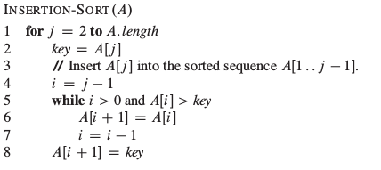
In this pseudocode, $A[j]$ is the ${j}^{th}$ element of the array $A$.

Let’s break the algorithm down:

The first line introduces a for loop, implying that the algorithm is gonna hold from elements 2 to the length of A.

The second line initialises key to A[j], which is initialsed to A[2] (again, keep in mind that A[2] in pseudocode is equivalent to A[1] in C/C++ code).

You might ask this question:

But dude, wait, doesn’t that mean that this algorithm doesn’t look for the first element?

Not exactly. The next few lines should convince you of it.

I’ll take the rest of this algorithm as one chunk of code (you’ll understand soon)

So, on the first try (or rather, iteration) of the algorithm, i becomes equal to j-1.

The next three lines just talk about how it is going to find the place for the key.

Once the place for it is found, key is placed in the element next to the place found, i.e., i+1.

Exercise: Find out why key is placed head of i by one element.

To have a more-or-less informal analysis of an algorithm, we need to know about loop invariants.

Correctness of Insertion Sort

For a quick-and-dirty version of its meaning, a loop invariant is something that retains its value over one iteration of the program, that is used for continuing the algorithm smoothly.

(Spoiler alert: The loop invariant for our implementation of insertion sort was j) The loop invariant helps to find if an algorithm is correct, or not.

We must show three things about a loop invariant:

Initialization: It is true prior to the first iteration of the loop.

Maintenance: If it is true before an iteration of the loop, it remains true before the next iteration.

Termination: When the loop terminates, the invariant gives us a useful property that helps show that the algorithm is correct.

Let’s see how this holds for insertion sort:

Initialization: Here, j=2, so the subarray A[1...j-1], therefore consists of A[1], and therefore, it is sorted.

Therefore, the loop invariant holds good at initialization.

Maintenance: This algorithm involves taking elements like A[j-1],A[j-2],A[j-3] etc. and moving them one by one till the element behind it is smaller than it. Therefore, A[1...j], where j is the place it the element gets placed is sorted.

(This part normally requires a good amount of math, but I am going to skip it, since this is an informal way to show correctness).

Termination: The condition that makes this algorithm exit is j=A.length, which means that A[1...A.length] is sorted by the time this algorithm is over. That is the whole algortihm.

Interesting Problems/Algorithms

• Prove the same for Bubblesort

More to come!

I will be posting the code of insertion sort, as well as the exercise solutions in a separate post tomorrow. Till then, try them and keep tuned!