Introduction to Algorithms - Chapter 2 (Part 2)

• Analysis of Algorithms
• Analysis of Insertion Sort
  • Finding Time Taken In Best Case
  • Finding Time Taken In Worst Case
• Divide And Conquer Principle
  • Merge Sort

Analysis of Algorithms

Analyzing an algorithm normally means predicting the resources that the algorithm requires.

Occasionally, resources such as memory, communication band- width, or computer hardware are of primary concern, but most often it is compu- tational time that we want to measure.

Okay, let’s do this!

(We assume here that the technology used for these algorithms here utilizes a generic one-processor, RAM (Random-Access Machine) model of computation)

Analysis of Insertion Sort

We can say that the time taken by the Insertion Sort Algorithm must be proportional to the time taken, since sorting 1000 numbers is more tedious than sorting 3 numbers.

Also, some implementations of insertion sort can be faster than the rest.

In general, since the time taken by an algorithm grows with the size of the input, it is traditional to describe the running time of a program as a function of the size of its input.

Therefore, we need to define “running time” and “size of input” more carefully.

The best notion for input size depends on the problem being studied. For many problems, such as sorting or computing discrete Fourier transforms, the most natural measure is the number of items in the input — for example, the array size n for sorting. For many other problems, such as multiplying two integers, the best measure of input size is the total number of bits needed to represent the input in ordinary binary notation. Sometimes, it is more appropriate to describe the size of the input with two numbers rather than one. For instance, if the input to an algorithm is a graph, the input size can be described by the numbers of vertices and edges in the graph. We shall indicate which input size measure is being used with each problem we study.

The running time of an algorithm on a particular input is the number of primitive operations or “steps” executed. It is convenient to define the notion of step so that it is as machine-independent as possible. For the moment, let us adopt the following view. A constant amount of time is required to execute each line of our pseudocode. One line may take a different amount of time than another line, but we shall assume that each execution of the ${i}^{th}$ line takes time $c_i$ , where $c_i$ is a constant. This viewpoint is in keeping with the RAM model, and it also reflects how the pseudocode would be implemented on most actual computers.

In the following discussion, our expression for the running time of Insertion Sort will evolve from a messy formula that uses all the statement costs $c_i$ to a much simpler notation that is more concise and more easily manipulated. This simpler notation will also make it easy to determine whether one algorithm is more efficient than another.

We start by presenting the Insertion Sort procedure with the time “cost” of each statement and the number of times each statement is executed. For each $j = 2,3,...,n$, where n = A:length, we let $t_j$ denote the number of times the while loop test in line 5 is executed for that value of j . When a for or while loop exits in the usual way (i.e., due to the test in the loop header), the test is executed one time more than the loop body. We assume that comments are not executable statements, and so they take no time.

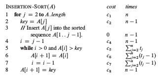
The total running time is the sum of running times for each statement executed. Therefore, the total time taken is:

So let’s find the best and worst cases, using which we will gain some insight as to how this algorithm works.

Finding Time Taken In Best Case

The best case in Insertion Sort obviously happens when the array is already sorted.

For all of $j = 2,3, \ldots,n$, we find that $A[i]\leq key $ in line 5 of the algorithm when i has an initial value of j - 1. Thus,$ t_j = 1 $for$ j = 2,3,/ldots,n $$ and the best-case running time is:

Since we can express it as $an + b$ for constants a and b, it is a linear function of n.

Finding Time Taken In Worst Case

The worst time happens when the summation terms are at their maximum.

Remembering that the summation terms can be simplified to:

and

We get:

We can express this time as $an^2 + bn + c$ for constants a, b, and c.

Therefore, it is a quadratic function of n.

Divide And Conquer Principle

This principle is used for problems which have subproblems that can be easily solved.

For example, if this sorting algorithm were to be fed only two elements at a time, it would be easy, right?

Therefore, if we can break down a problem to small, easily solvable chunks, solving the problem becomes easier. Just make the real problem by solving all the bits and pieces!

This is a complex skill, worth it’s own page (which I will give), but let’s see it in action first.

Merge Sort

This is the code for mergesort:

// Merge Sort

#include <iostream>
using namespace std;

int a[50];
void merge(int,int,int);
void merge_sort(int low,int high)
{
 if(low<high)
 {
  int mid = low + (high-low)/2; //This avoids overflow when low, high are too large
  merge_sort(low,mid);
  merge_sort(mid+1,high);
  merge(low,mid,high);
 }
}
void merge(int low,int mid,int high)
{
 int h,i,j,b[50],k;
 h=low;
 i=low;
 j=mid+1;

 while((h<=mid)&&(j<=high))
 {
  if(a[h]<=a[j])
  {
   b[i]=a[h];
   h++;
  }
  else
  {
   b[i]=a[j];
   j++;
  }
  i++;
 }
 if(h>mid)
 {
  for(k=j;k<=high;k++)
  {
   b[i]=a[k];
   i++;
  }
 }
 else
 {
  for(k=h;k<=mid;k++)
  {
   b[i]=a[k];
   i++;
  }
 }
 for(k=low;k<=high;k++) a[k]=b[k];
}
int main()
{
 int num,i;
 cout<<"Please Enter THE NUMBER OF ELEMENTS you want to sort [THEN 
PRESS
ENTER]:"<<endl;
 cin>>num;
 cout<<"\n Now, Please Enter the ( "<< num <<" ) numbers (ELEMENTS) [THEN
PRESS ENTER]:"<<endl;
 for(i=1;i<=num;i++)
 {
  cin>>a[i] ;
 }
 merge_sort(1,num);
 cout<<endl;
 cout<<"So, the sorted list (using MERGE SORT) will be :"<<endl;
 cout<<endl<<endl;

 for(i=1;i<=num;i++)
 cout<<a[i]<<"  ";

}

Try to understand it. I’ll explain it in the next post.